Data reduction#
Introduction#
The documentation on this page contains an introduction into data reduction of the modified VLT/VISIR instrument for the NEAR (New Earths in the Alpha Cen Region) experiment. All data are available in the ESO archive under program ID 2102.C-5011(A).
The basic processing steps with PynPoint are described in the example below while a complete overview of all available pipeline modules can be found in the Pipeline modules section. Further details about the pipeline architecture and data processing are also available in Stolker et al. (2019). More in-depth information of the input parameters for individual PynPoint modules can be found in the API Documentation.
Please also have a look at the Attribution section when using PynPoint results in a publication.
Example#
In this example, we will process the images of chop A (i.e., frames in which alpha Cen A was centered behind the AGPM coronagraph). Note that the same procedure can be applied on the images of chop B (i.e., with alpha Cen B centered behind the coronagraph).
Setup#
To get started, use the instructions available in the Installation section to install PynPoint. We also need to download the NEAR data associated with the ESO program that was provided above. It is recommended to start with downloading only a few files to first validate the pipeline installation.
Now that we have the data, we can start the data reduction with PynPoint!
The Pypeline of PynPoint requires a folder for the working_place, input_place, and output_place. Before we start running PynPoint, we have to put the raw NEAR data in the default input folder or the location that will provided as input_dir in the NearReadingModule.
Then we create a configuration file which contains the global pipeline settings and is used to select the required FITS header keywords. Create a text file called PynPoint_config.ini in the working_place folder with the following content:
[header]

INSTRUMENT: INSTRUME
NFRAMES: ESO DET CHOP NCYCLES
EXP_NO: ESO TPL EXPNO
DIT: ESO DET SEQ1 DIT
NDIT: None
PARANG_START: ESO ADA POSANG
PARANG_END: ESO ADA POSANG END
DITHER_X: None
DITHER_Y: None
PUPIL: ESO ADA PUPILPOS
DATE: DATE-OBS
LATITUDE: ESO TEL GEOLAT
LONGITUDE: ESO TEL GEOLON
RA: RA
DEC: DEC

[settings]

PIXSCALE: 0.045
MEMORY: 1000
CPU: 1
The MEMORY and CPU setting can be adjusted. They define the number of images that is simultaneously loaded into the computer memory and the number of parallel processes that are used by some of the pipeline modules.
Note that in addition to the config file above, the working_place directory is also used to store the database file (PynPoint_database.hdf5). This database stores all intermediate results (typically a stack of images), which allows the user to rerun particular processing steps without having to rerun the complete pipeline.
Running PynPoint#
Example code snippets for the different steps to reduce NEAR data with PynPoint are included below. These code snippets can be executed in Python interactive mode, as a Jupyter notebook.py file, or combined into a python script and executed from the command line.
The first steps are to initialize the pipeline and read in the data contained in the given input_place_in directory. Data are automatically divided into the chop A and chop B data sets. Here we also use the AngleInterpolationModule to calculate the parallactic angle for each individual frame, which is necessary for derotating and combining the frames after PSF subtraction:
# Import the Pypeline and the modules that we will use in this example

from pynpoint import Pypeline, NearReadingModule, AngleInterpolationModule, \
                     CropImagesModule, SubtractImagesModule, ExtractBinaryModule, \
                     StarAlignmentModule, FitCenterModule, ShiftImagesModule, \
                     FakePlanetModule, PSFpreparationModule, PcaPsfSubtractionModule, \
                     ContrastCurveModule, FitsWritingModule, TextWritingModule

# Create a Pypeline instance (change the directories to the correct paths)

pipeline = Pypeline(working_place_in='working_folder/',  # directory for database and config files
                    input_place_in='input_folder/',      # default directory for reading in input data
                    output_place_in='output_folder/')    # default directory for saving output files
                                                         #   (i.e., with FitsWritingModule used below)

# Read the raw data (i.e., all the fits files contained in the input_place_in folder above)
# and separate the chop A and chop B images

module = NearReadingModule(name_in='read',
                           input_dir=None,
                           chopa_out_tag='chopa',
                           chopb_out_tag='chopb')

pipeline.add_module(module)

# Interpolate the parallactic angles between the start and end value of each FITS file
# The angles will be added as PARANG attribute to the chop A and chop B datasets

module = AngleInterpolationModule(name_in='angle1',
                                  data_tag='chopa')

pipeline.add_module(module)

module = AngleInterpolationModule(name_in='angle2',
                                  data_tag='chopb')

pipeline.add_module(module)

# Run each of the above modules using their 'name_in' tags

pipeline.run_module('read')
pipeline.run_module('angle1')
pipeline.run_module('angle2')

# Note that you can also run all the added modules using this function:
# pipeline.run()
The next step is to reduce the chop A frames with alpha Cen A behind the corognagraph. Here we crop the chop A and chop B images around the coronagraph position, subtract chop B from chop A to remove the sky background, and center the subtracted chop A frames:
# Crop the chop A and chop B images around the approximate coronagraph position

module = CropImagesModule(size=5.,
                          center=(432, 287),
                          name_in='crop1',
                          image_in_tag='chopa',
                          image_out_tag='chopa_crop')

pipeline.add_module(module)

module = CropImagesModule(size=5.,
                          center=(432, 287),
                          name_in='crop2',
                          image_in_tag='chopb',
                          image_out_tag='chopb_crop')

pipeline.add_module(module)

# Subtract frame-by-frame chop B from chop A

module = SubtractImagesModule(name_in='subtract_aminusb',
                              image_in_tags=('chopa_crop', 'chopb_crop'),
                              image_out_tag='chopa_sub',
                              scaling=1.)

pipeline.add_module(module)

# Fit the center position of chop A, using the images from before the chop-subtraction
# For simplicity, only the mean of all images is fitted

module = FitCenterModule(name_in='center1',
                         image_in_tag='chopa_crop',
                         fit_out_tag='chopa_fit',
                         mask_out_tag=None,
                         method='mean',
                         radius=1.,
                         sign='positive',
                         model='moffat',
                         filter_size=None,
                         guess=(0., 0., 10., 10., 1e4, 0., 0., 1.))

pipeline.add_module(module)


# Center the chop-subtracted images

module = ShiftImagesModule(shift_xy='chopa_fit',
                           name_in='shift1',
                           image_in_tag='chopa_sub',
                           image_out_tag='chopa_center',
                           interpolation='spline')

pipeline.add_module(module)

# Run each of the above modules

pipeline.run_module('crop1')
pipeline.run_module('crop2')
pipeline.run_module('subtract_aminusb')
pipeline.run_module('center1')
pipeline.run_module('shift1')
Next, we use the chop B frames where alpha Cen A if off of the coronagraph to extract a reference PSF. This reference PSF will later be used for calculating the detection limits:
# Subtract chop A from chop B before extracting the non-coronagraphic PSF

module = SubtractImagesModule(name_in='subtract_bminusa',
                              image_in_tags=('chopb', 'chopa'),
                              image_out_tag='chopb_sub',
                              scaling=1.)

pipeline.add_module(module)

# Crop out the non-coronagraphic PSF for chop A from the chop B images

module = ExtractBinaryModule(pos_center=(432., 287.),
                             pos_binary=(430., 175.),
                             name_in='extract_refpsf',
                             image_in_tag='chopb_sub',
                             image_out_tag='psfa',
                             image_size=5.,
                             search_size=1.,
                             filter_size=None)

pipeline.add_module(module)

# Align the non-coronagraphic PSF images

module = StarAlignmentModule(name_in='align_refpsf',
                             image_in_tag='psfa',
                             ref_image_in_tag=None,
                             image_out_tag='psfa_align',
                             interpolation='spline',
                             accuracy=10,
                             resize=None,
                             num_references=10,
                             subframe=1.)

pipeline.add_module(module)

# Fit the center position of the mean, non-coronagraphic PSF

module = FitCenterModule(name_in='center_refpsf',
                         image_in_tag='psfa',
                         fit_out_tag='psfa_fit',
                         mask_out_tag=None,
                         method='mean',
                         radius=1.,
                         sign='positive',
                         model='moffat',
                         filter_size=None,
                         guess=(0., 0., 10., 10., 1e4, 0., 0., 1.))

pipeline.add_module(module)

# Center the non-coronagraphic PSF images

module = ShiftImagesModule(shift_xy='psfa_fit',
                           name_in='shift_refpsf',
                           image_in_tag='psfa',
                           image_out_tag='psfa_center',
                           interpolation='spline')

pipeline.add_module(module)

# Mask the non-coronagraphic PSF beyond 1 arsec

module = PSFpreparationModule(name_in='prep_refpsf',
                              image_in_tag='psfa_center',
                              image_out_tag='psfa_mask',
                              mask_out_tag=None,
                              norm=False,
                              cent_size=None,
                              edge_size=1.)

pipeline.add_module(module)

# Run each of the above modules

pipeline.run_module('subtract_bminusa')
pipeline.run_module('extract_refpsf')
pipeline.run_module('align_refpsf')
pipeline.run_module('center_refpsf')
pipeline.run_module('shift_refpsf')
pipeline.run_module('prep_refpsf')
Finally, we use PCA to subtract the stellar PSF of alpha Cen A. For testing purposes, we first use the reference PSF created above to inject a fake planet into the chop A data. The median combination of the PSF-subtracted and derotated frames is saved in its own tag and then written out to a fits file:
# Inject a fake planet at a separation of 1 arcsec and a contrast of 10 mag

module = FakePlanetModule(position=(1., 0.),
                          magnitude=10.,
                          psf_scaling=1.,
                          interpolation='spline',
                          name_in='fake',
                          image_in_tag='chopa_center',
                          psf_in_tag='psfa_mask',
                          image_out_tag='chopa_fake')

pipeline.add_module(module)

# Mask the central and outer part of the chop A images

module = PSFpreparationModule(name_in='prep_data',
                              image_in_tag='chopa_fake',
                              image_out_tag='chopa_prep',
                              mask_out_tag=None,
                              norm=False,
                              cent_size=0.3,
                              edge_size=3.)

pipeline.add_module(module)

# Subtract a PSF model with PCA and median-combine the residuals

module = PcaPsfSubtractionModule(pca_numbers=range(1, 51),
                                 name_in='pca',
                                 images_in_tag='chopa_prep',
                                 reference_in_tag='chopa_prep',
                                 res_median_tag='chopa_pca',
                                 extra_rot=0.0)

pipeline.add_module(module)

# Datasets can be exported to FITS files by their tag name in the database
# Here we will export the median-combined residuals of the PSF subtraction

module = FitsWritingModule(name_in='write_result_psfsub',
                           file_name='chopa_pca.fits',
                           output_dir=None,
                           data_tag='chopa_pca',
                           data_range=None,
                           overwrite=True)

pipeline.add_module(module)

# Run each of the above modules

pipeline.run_module('fake')
pipeline.run_module('prep_data')
pipeline.run_module('pca')
pipeline.run_module('write_result_psfsub')
PynPoint also includes a module to calculate the detection limits of the final image:
# Calculate detection limits between 0.8 and 2.0 arcsec
# The false positive fraction is fixed to 2.87e-6 (i.e. 5 sigma for Gaussian statistics)

module = ContrastCurveModule(name_in='limits',
                             image_in_tag='chopa_center',
                             psf_in_tag='psfa_mask',
                             contrast_out_tag='limits',
                             separation=(0.3, 2., 0.1),
                             angle=(0., 360., 60.),
                             threshold=('fpf', 2.87e-6),
                             psf_scaling=1.,
                             aperture=0.15,
                             pca_number=10,
                             cent_size=0.3,
                             edge_size=3.,
                             extra_rot=0.,
                             residuals='median')

pipeline.add_module(module)

# And we write the detection limits to a text file

header = 'Separation [arcsec] - Contrast [mag] - Variance [mag] - FPF'

module = TextWritingModule(name_in='write_result_limits',
                           file_name='contrast_curve.dat',
                           output_dir=None,
                           data_tag='limits',
                           header=header)

pipeline.add_module(module)

# Run each of the above modules

pipeline.run_module('limits')
pipeline.run_module('write_result_limits')
Results#
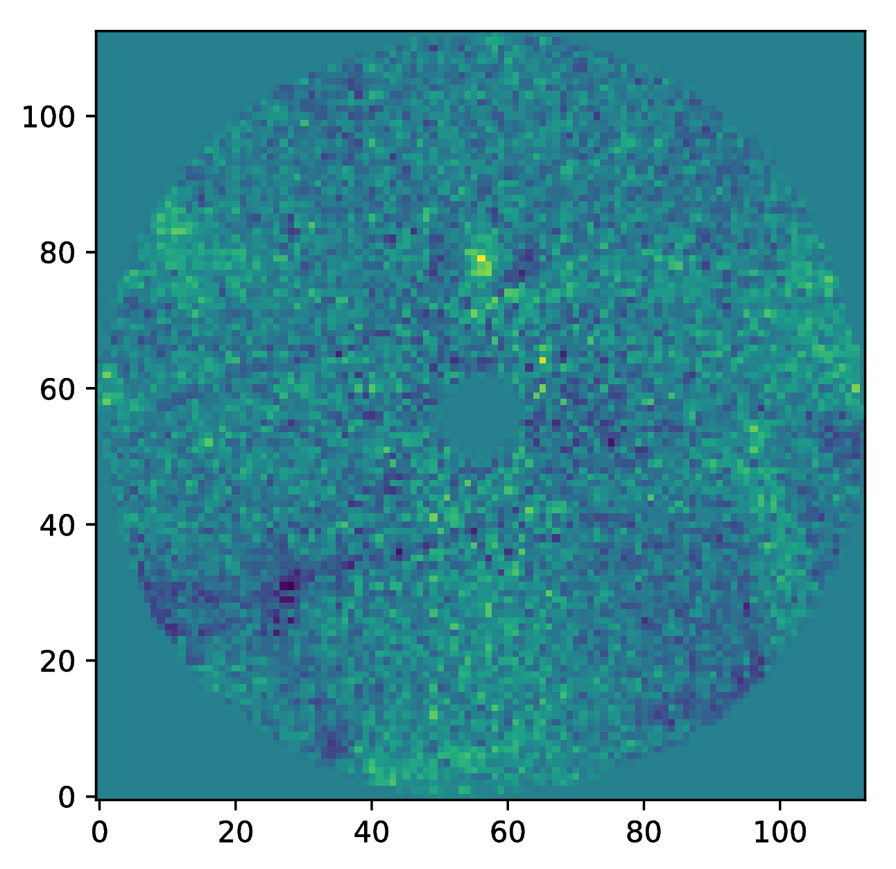
The images that were exported to a FITS file can be visualized with a tool such as DS9. We can also use the Pypeline functionalities to get the data from the database (without having to rerun the pipeline). For example, to get the residuals of the PSF subtraction:
data = pipeline.get_data('chopa_pca')
And to plot the residuals for 10 principal components (Python indexing starts at zero):
import matplotlib.pyplot as plt

plt.imshow(data[9, ], origin='lower')
plt.show()
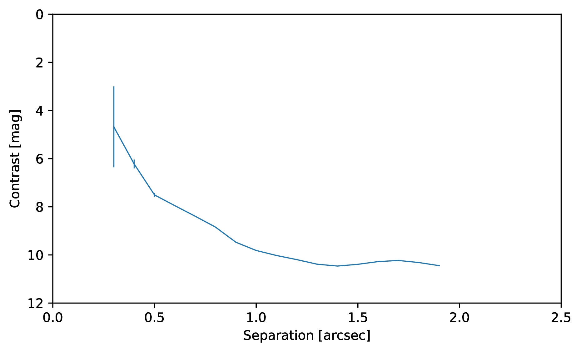
Or to plot the detection limits with the error bars showing the variance of the six azimuthal positions that were tested:
data = pipeline.get_data('limits')

plt.figure(figsize=(7, 4))
plt.errorbar(data[:, 0], data[:, 1], data[:, 2])
plt.xlim(0., 2.5)
plt.ylim(12., 0.)
plt.xlabel('Separation [arcsec]')
plt.ylabel('Contrast [mag]')
plt.show()